
Is Cristiano Ronaldo lost his interest in twitter? A fun analysis of tweets of Cristiano Ronaldo using R
Arun Gopinath / 2021-11-21
- A detailed analysis of tweets of famous footballer Cristiano Ronaldo in R
- Let’s dive into it.
- Is there any pattern over the months ?
- What about over the days ?
- Tweets over the time
- Retweets v/s Original tweets
- Text mining - Let’s deep dive into the tweet data
- Create a wordcloud using the words used in his tweets so far.
- Conclusion
A detailed analysis of tweets of famous footballer Cristiano Ronaldo in R
In this post we are going to have a quick roundup of Cristiano Ronaldo’s tweets. For this mission various powerful tools of ‘R’ are used.
library(rtweet)
library(tidyverse)
library(lubridate)
library(hms)
library(scales)
library(tidytext)
library(wordcloud)
library(syuzhet)
Get Ronaldo’s tweets timeline
Due to limitations of twitter new policy, we can only retrieve last 3200 tweets of a user. In our case, as of writing this article his total tweets are just 3733. So we are covering most of his twitter journey here.
Ronaldo <- get_timeline("@cristiano", n= 3200)Let’s dive into it.
Plotting tweets per months over the time period
As the first user case lets see how he tweets over these years.
ggplot(data = Ronaldo,
       aes(month(created_at, label=TRUE, abbr=TRUE),
           group=factor(year(created_at)), color=factor(year(created_at))))+
  geom_line(stat= "count") +
  geom_point(stat="count") +
  labs(x="Month", colour="Year", xlab = "Month", ylab = "Number of tweets",
       title = "Cristiano Ronaldo's tweets over the time period",
       caption = "Created by Arun Gopinath") +
  theme_minimal()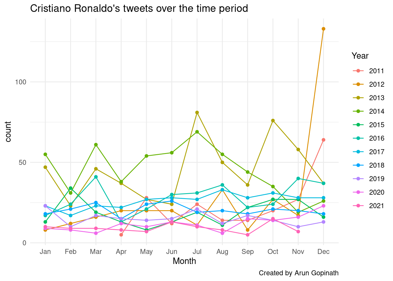
It’s quite difficult to obtain a trend here. But one thing is sure, his interest in twitter is just fading away.
Bar plot to get more insight
ggplot(data = Ronaldo, aes(x = year(created_at))) +
  geom_bar(aes(fill = ..count..)) +
  xlab("Year") + ylab("Number of tweets") +
  labs(title = "Cristiano Ronaldo's tweets over the time period",
       subtitle = "2013 & 2014 been his prime time in twitter",
       caption = "Created by Arun Gopinath")+
  scale_x_continuous (breaks = c(2010:2021)) +
  theme_minimal() +
  scale_fill_gradient(low = "yellow", high = "darkgreen")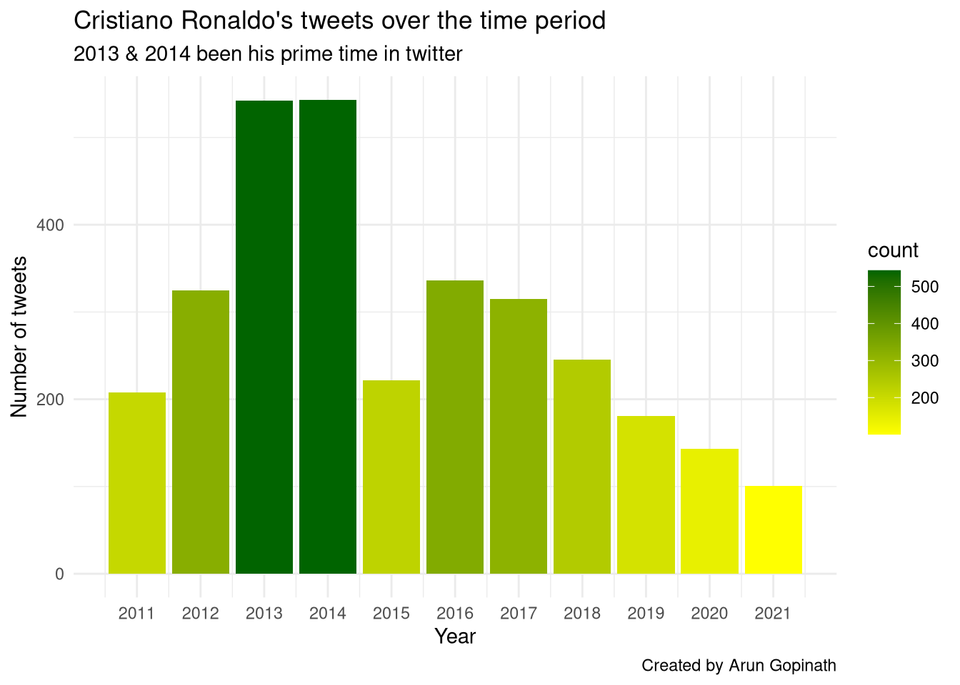
Is there any pattern over the months ?
ggplot(data = Ronaldo, aes(x = month(created_at, label = TRUE))) +
  geom_bar(aes(fill = ..count..)) +
  xlab("Month") + ylab("Number of tweets") +
  labs(title = "Cristiano Ronaldo's tweets - Monthwise",
       subtitle = "It's december",
       caption = "Created by Arun Gopinath")+
  theme_minimal() +
  scale_fill_gradient(low = "yellow", high = "red")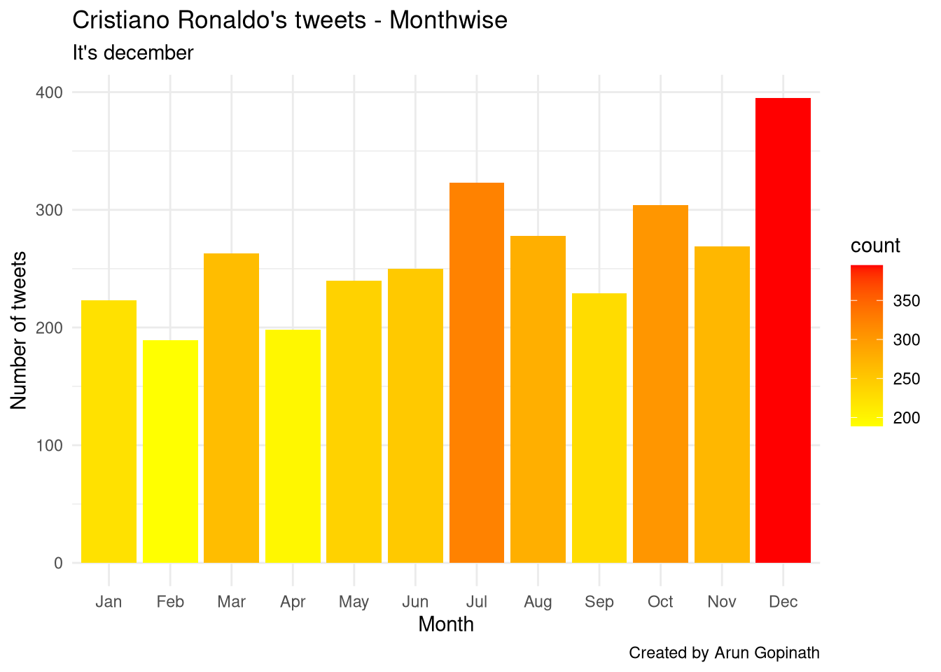
What about over the days ?
ggplot(data = Ronaldo, aes(x = wday(created_at, label = TRUE))) +
  geom_bar(aes(fill = ..count..)) +
  xlab("Day of the week") + ylab("Number of tweets") +
  labs(title = "Do you know which day Cristiano Ronaldo pick to tweet least ?",
       subtitle = "Weekends are holidays",
       caption = "Created by Arun Gopinath")+
  theme_minimal() +
  scale_fill_gradient(low = "turquoise3", high = "darkgreen")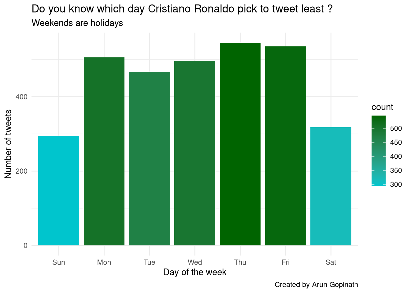
Sundays are usually his least tweeted day so far. While Thursdays are more engaged one.
Tweets over the time
Let’s look another factor which may influence his tweet pattern - Time during a day.
But our date and time are in combined form so clean it up using hms and scales packages as given below.
## Get hour, minute and seconds from tweets

Ronaldo$time <- hms::hms(second(Ronaldo$created_at),
                           minute(Ronaldo$created_at),
                           hour(Ronaldo$created_at))

## Converting to `POSIXct` as ggplot isn’t compatible with `hms`
Ronaldo$time <- as.POSIXct(Ronaldo$time)
Our data is ready to plot. Any guess ?
ggplot(data = Ronaldo)+
  geom_density(aes(x = time, y = ..scaled..),
               fill="steelblue", alpha=0.3) +
  xlab("Time") + ylab("Density") +
  labs(title = "Cristiano Ronaldo tweet pattern",
       subtitle = "His sleeping pattern is quite good !",
       caption = "Created by Arun Gopinath")+
  scale_x_datetime(breaks = date_breaks("2 hours"),
                   labels = date_format("%H:%M")) +
  theme_minimal()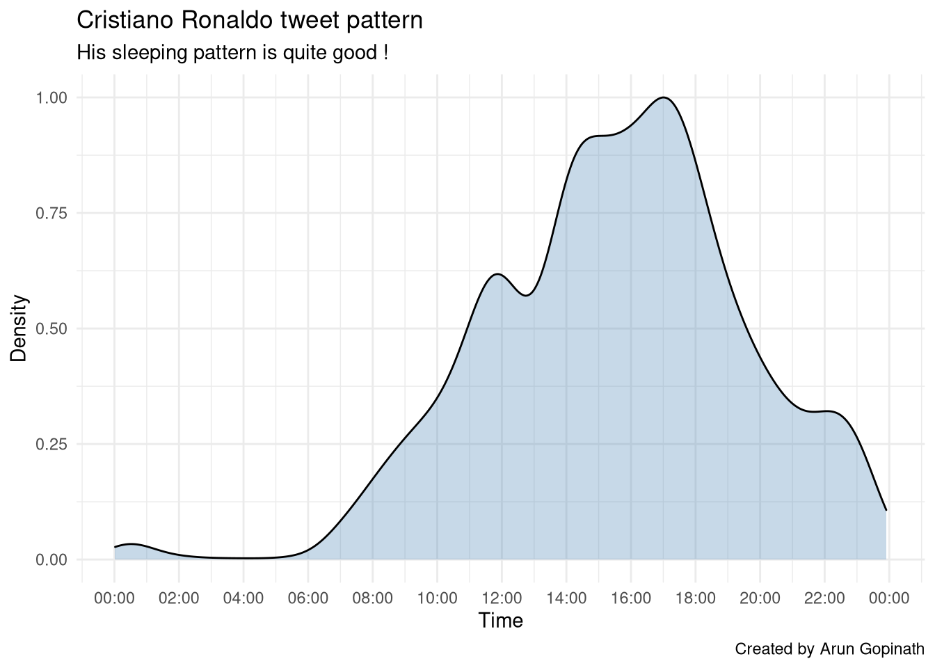
As expected from a super player like Ronaldo, his twitter usage is negligible between 12 am and 6 am. Another reason for his super powers on the field. Also he spends more time online during evening section.
Retweets v/s Original tweets
Do Ronaldo retweet more nowadays?
ggplot(data = Ronaldo, aes(x = created_at, fill = is_retweet)) +
  geom_histogram(bins=30) +
  xlab("Time") + ylab("Number of tweets") +
  labs(title = "Cristiano Ronaldo's Retweets v/s Original tweets",
       subtitle = "Almost stopped retweeting after 2015 !",
       caption = "Created by Arun Gopinath")+
  theme_minimal() +
  scale_fill_manual(values = c("darkolivegreen3", "darkolivegreen4"), name = "Retweet")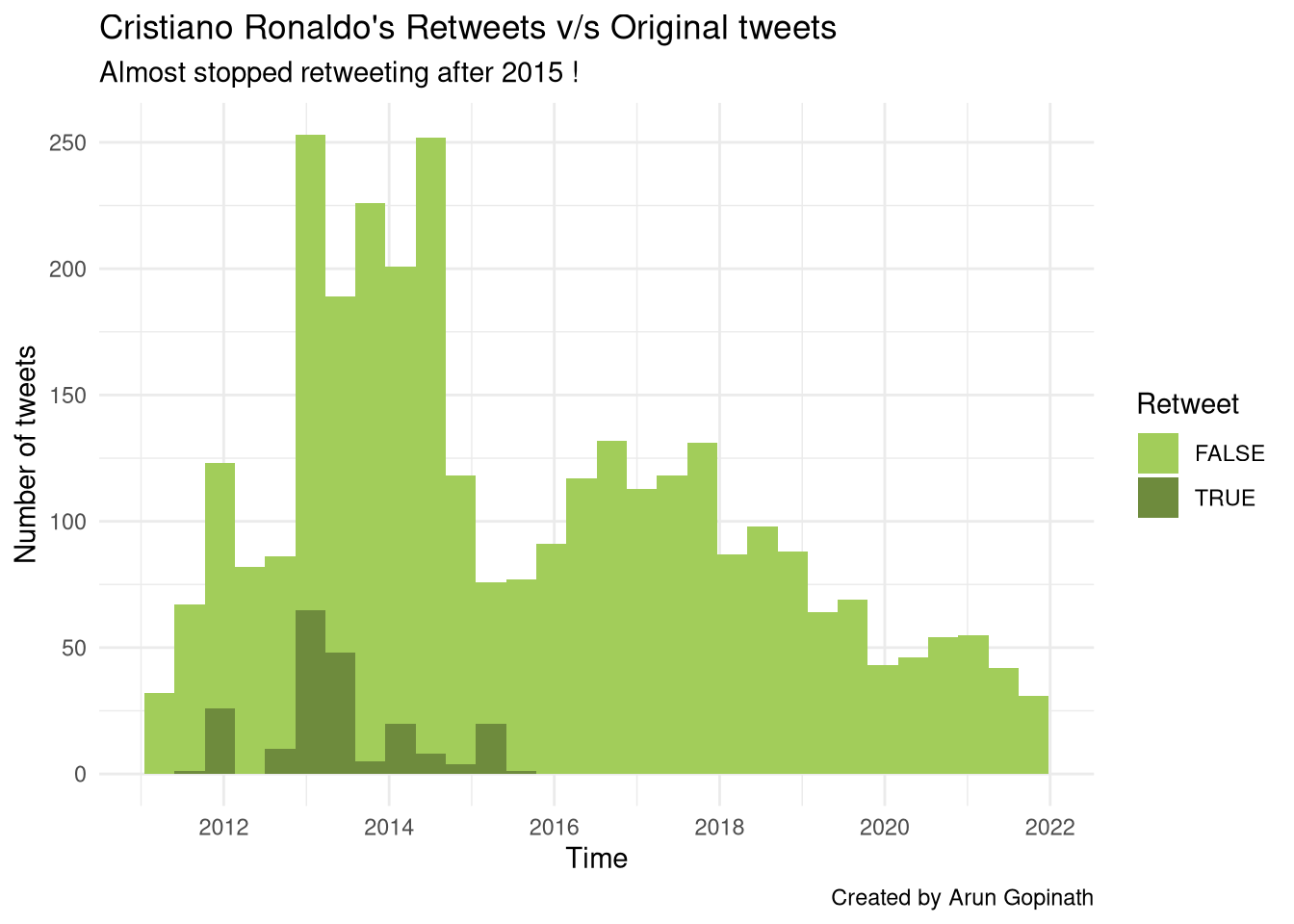
No not at all !!
Text mining - Let’s deep dive into the tweet data
What about Hashtags frequency ?
What are the top 10 hashtags he tweeted ?
Ronaldo %>%
  unnest_tokens(hashtag, text, "tweets", to_lower = FALSE) %>%
  filter(str_detect(hashtag, "^#")) %>%
  count(hashtag, sort = TRUE) %>%
  top_n(10) %>%
  ggplot(aes(x = reorder(hashtag, -n), y =n))+
  geom_segment( aes(xend=hashtag, yend=0)) +
  geom_point( size=4, color="red") +
  theme_bw() +
  ylab("Count")+
  xlab("Hashtags")+
  labs(title = "Cristiano Ronaldo's top 10 twitter #hashtags",
       subtitle = "",
       caption = "Created by Arun Gopinath")+
  coord_flip()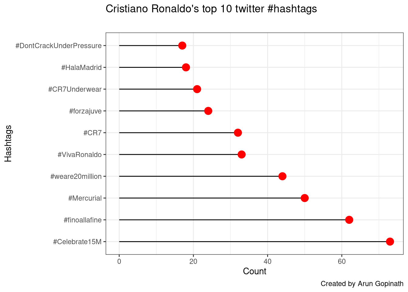
Most of them are sports related, especially about teams he represented and his personal milestones.
Most retweeted tweet
Which tweet is the most retweeted tweet ?
Ronaldo %>%
  arrange(-retweet_count) %>%
  slice(1) %>%
  select(created_at, screen_name, text, retweet_count, status_id)
So happy to be able to hold the two new loves of my life 🙏❤ pic.twitter.com/FIY11aWQm9
— Cristiano Ronaldo (@Cristiano) June 29, 2017
Most liked tweet
Ronaldo %>%
  arrange(-favorite_count) %>%
  top_n(5, favorite_count) %>%
  select(created_at, screen_name, text, favorite_count)
So sad to hear the heartbreaking news of the deaths of Kobe and his daughter Gianna. Kobe was a true legend and inspiration to so many. Sending my condolences to his family and friends and the families of all who lost their lives in the crash. RIP Legend💔 pic.twitter.com/qKb3oiDHxH
— Cristiano Ronaldo (@Cristiano) January 26, 2020
Top mentions
Ronaldo %>%
  unnest_tokens(mentions, text, "tweets", to_lower = FALSE) %>%
  filter(str_detect(mentions, "^@")) %>%
  count(mentions, sort = TRUE) %>%
  top_n(10)
## # A tibble: 10 x 2
## mentions n
## <chr> <int>
## 1 @Cristiano 177
## 2 @nikefootball 54
## 3 @GAMEbyRonaldo 37
## 4 @realmadrid 25
## 5 @VivaRonaldo 25
## 6 @cristiano 18
## 7 @TAGHeuer 17
## 8 @Herbalife 16
## 9 @SavetheChildren 16
## 10 @HeadsUp 13Create a wordcloud using the words used in his tweets so far.
Find top words
Here we want to remove white spaces, symbols, signs etc. Also remove stop words, words which are frequently used by everyone, from the list.And finally sort it 1.
words <- Ronaldo %>%
mutate(text = str_remove_all(text, "&|<|>"),
text = str_remove_all(text, "\\s?(f|ht)(tp)(s?)(://)([^\\.]*)[\\.|/](\\S*)"),
text = str_remove_all(text, "[^\x01-\x7F]")) %>%
unnest_tokens(word, text, token = "tweets") %>%
filter(!word %in% stop_words$word,
!word %in% str_remove_all(stop_words$word, "'"),
str_detect(word, "[a-z]"),
!str_detect(word, "^#"),
!str_detect(word, "@\\S+")) %>%
count(word, sort = TRUE)Wordcloud
Now plot a wordcloud from what we got.
set.seed(1234)

words %>%
  with(wordcloud(word, n, random.order = FALSE, max.words = 150,
                 scale=c(2.6,0.25),colors=brewer.pal(8, "Dark2")))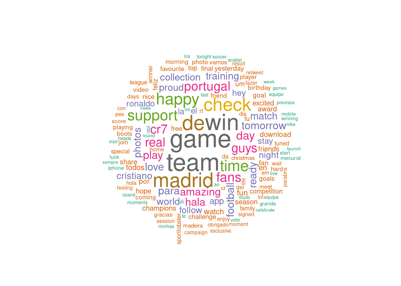
Sentiment analysis
Sentiment analysis (or opinion mining) is a natural language processing (NLP) technique used to determine whether data is positive, negative or neutral. Sentiment analysis is often performed on textual data to help businesses monitor brand and product sentiment in customer feedback, and understand customer needs2.
Here we analyse 10 emotions from positive to disgust.
- First convert text to ASCII to tackle strange characters like what we done above.
tweet_text <- iconv(words, from="UTF-8", to="ASCII", sub="")- Since we are playing with tweets of Ronaldo ignore retweets.
Tweet_text <- gsub("(RT|via)((?:\\b\\w*@\\w+)+)","",tweet_text)- Also remove mentions
Tweet_text <- gsub("@\\w+","",tweet_text)- Get sentiment score using ‘get_nrc_sentiment’ function.
Ron_sentiment <- get_nrc_sentiment((tweet_text))- To display it in ggplot we want to convert it into a data frame.
Sentimentscores <- data.frame(colSums(Ron_sentiment[,]))- For better understanding of data frame better headers are assigned.
names(Sentimentscores) <- "Score"
Sentimentscores <- cbind("sentiment"=rownames(Sentimentscores),Sentimentscores)
rownames(Sentimentscores) <- NULL
Sentiment plot
Finally our sentiment plot of Cristiano Ronaldo’s tweets 3.
ggplot(data=Sentimentscores,aes(x=sentiment,y=Score))+
  geom_bar(aes(fill=sentiment),stat = "identity")+
  theme(legend.position="none")+
  xlab("Sentiments")+ylab("Scores")+
  labs(title = "Total sentiment of Cristiano Ronaldo's tweets based on scores",
       subtitle = "Positive vibes")+
  theme(axis.text.x = element_text(angle = 90, vjust = 0.5, hjust=1))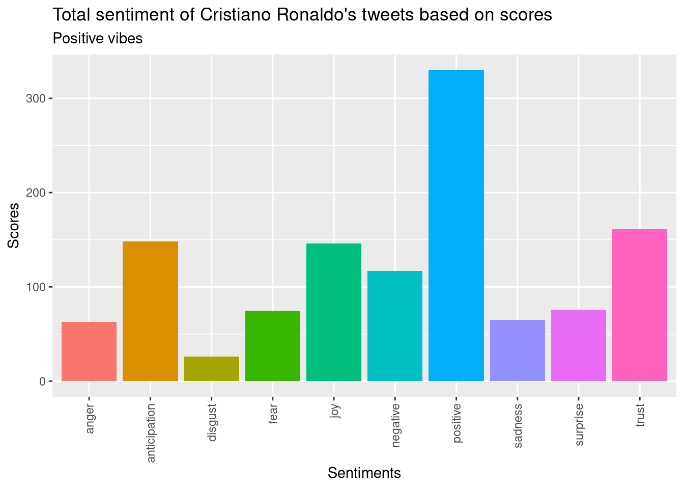
- Positive vibes overall.
Conclusion
Cristiano Ronaldo is shifting his gears with new age social media like Instagram. Tweet frequency is dramatically getting lower over the years.Further analysis can be done based to mine more and more intersting details. Happy mining.