Can you identify this legendary malayalam novel ? A ggwordcloud experiment in R

Arun Gopinath / 2021-06-17

A legendary novel

Yesterday out of nowhere the masterpiece novel, which changed the course of Malayalam literature forever pop up in my social media feed. After reading the digital copy (.epub) of the same, the idea for this article came into my mind. All I have for you is “words”.

Create a word cloud using R

First of all, load necessary R packages. {readtext} and {tidytext} for load our novel. {tidyverse} - the most important package for data wrangling. {ggplot2} and {ggwordcloud} for visualisation.

library(tidytext)
library(readtext)
library(here)
library(tidyverse)
library(ggplot2)
library(ggwordcloud)

Load files

Load files. (If you follow the clue, you are already in the right direction to find this masterpiece novel). Here, the novel is in ‘.txt’ format. “unnest_token” will convert the entire file into a two-column table.

k <- readtext(here("static/data","k.txt"))
token_k <- k %>% unnest_tokens(word,text)

Little bit data wrangling

We are almost there. The only thing we want to visualise is nothing but the word count. “count(word,sort = TRUE)” will get the job done for us. For tidiness of the plot count greater than “25” is used (Who loves messy visuals?). As a final step,{ggwordcloud} is applied with suitable text size, colour. The benefit of {ggwordcloud} is its integration with {ggplot2} outputs. For cooler representation some tilting of words are also included and stored in a new coloumn named “angle”.

wcloud <- token_k %>% 
  count(word,sort = TRUE) %>% 
  filter(n > 25) %>%  
  mutate(word = reorder(word,n)) %>% 
  mutate(angle = 45 * sample(-2:2, n(), replace = TRUE, prob = c(1, 1, 4, 1, 1)))

Final step - Visualisation

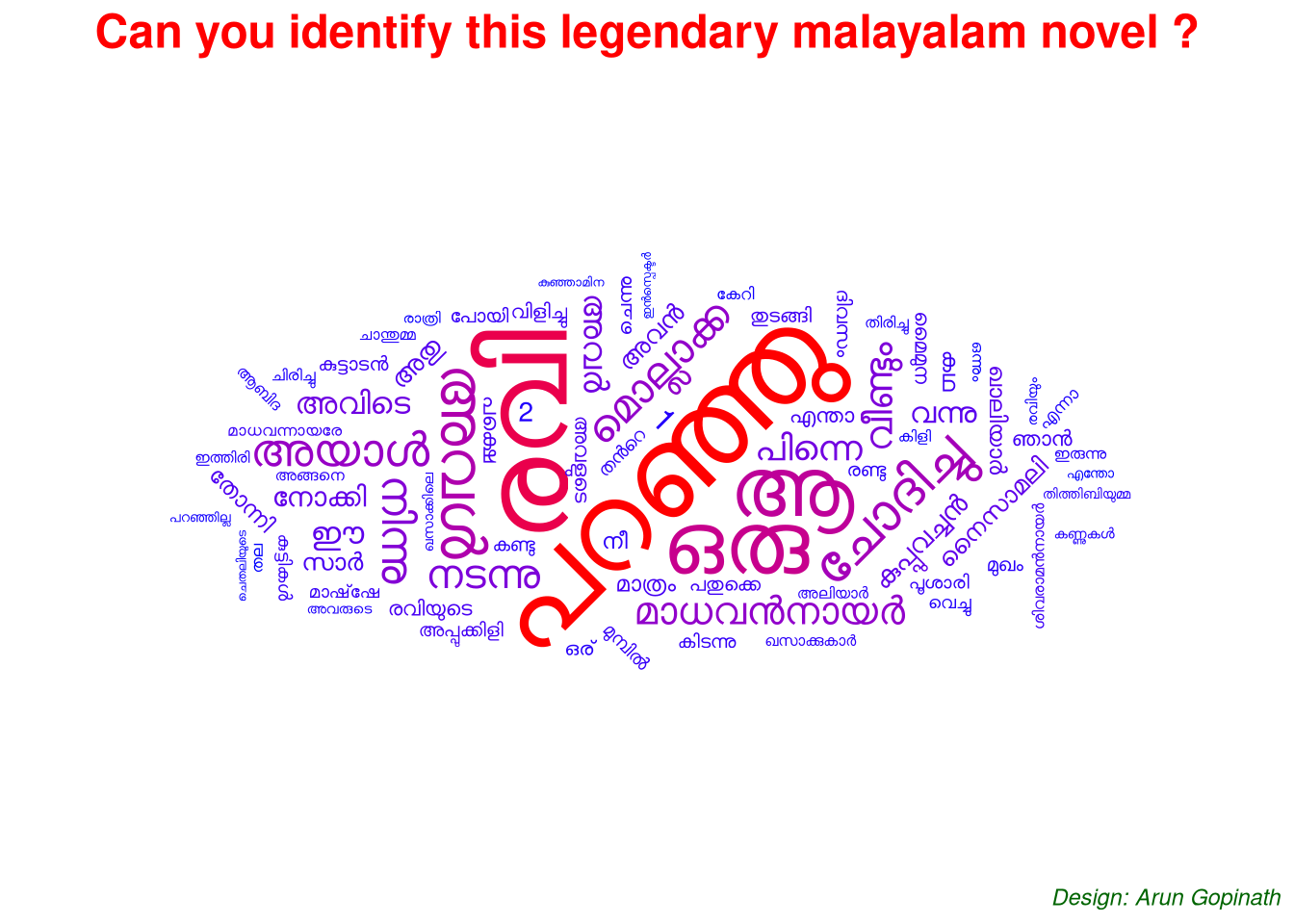
In the visualisation step, {ggplot} is used along with “geom_text_wordcloud_area” function in {ggwordcloud}. Colour is based on the frequency of words in the file. Also, most frequent words are set to “red” and less frequent ones to “blue”. Finally, a cool title and caption are added (Theme section)

set.seed(42)
kplot <- ggplot(wcloud, aes(label = word,size =n, angle = angle,
                            color = n)) +
   geom_text_wordcloud_area() +
  scale_size_area(max_size = 20) +
  
  # theme section
  theme_minimal()+
  scale_colour_gradient(low = "blue", high = "red", na.value = NA)+
  
  # title and caption
  labs(
    title = "Can you identify this legendary malayalam novel ?",
    caption = "Design: Arun Gopinath"
  )+
  theme(
  plot.title = element_text(color = "red", size = 18, face = "bold",hjust = 0.5),
  plot.caption = element_text(color = "darkgreen", face = "italic")
)
kplot